An open wind tunnel is a wind tunnel that takes in air from the surroundings, and outputs it to the surroundings. This is in contrast to a closed wind tunnel, which recirculates the air (i.e. the outlet is connected to the inlet). The difference is mainly power savings.
This article will describe the boundary conditions necessary to simulate an open wind tunnel.
An important thing to realize is that static pressure in a wind tunnel is not constant from upstream to downstream, as it is for an actual vehicle in flight. The small but significant pressure gradient is required to create a flow and is created by the fan powering the wind tunnel (fans produce a pressure gradient, which is how they provide thrust).
Often in aerodynamics, because the air is invisible, many flow properties are indirectly measured. Wind tunnel velocity is typically measured by dynamic pressure, which is the additional pressure generated when a moving flow comes to a halt. For incompressible flows (below about Mach 0.3), the dynamic pressure can be calculated by 0.5*density*velocity^2.
Knowing this we can set up proper boundary conditions for an open wind tunnel. The following are the boundary conditions for U (velocity) and p (pressure). Set the desired wind tunnel velocity to V.
Walls: U = 0, p = zero gradient
Inlet: U = zero gradient, p = zero gradient, p0 (total pressure) = 1/2*density*V^2
Outlet: U = zero gradient, p = 0
Thursday, November 22, 2012
Sunday, November 11, 2012
Getting Started with GPU Coding: CUDA 5.0
Hello everyone, this is a quick post detailing how to get started with harnessing the potential of your GPU via CUDA. Of course, I am planning to use it for OpenFOAM; I want to translate the pimpleDyMFoam solver for CUDA.
Especially awesome about CUDA 5.0 is the new Nsight IDE for Eclipse. If you have ever programmed with Eclipse (I have in Java), you know how spoiled you can get with all of the real-time automated correction and prediction.
Anyways, here are the steps I took:
I have Ubuntu 12.04, and even though the CUDA toolkit web page has only downloads for Ubuntu 11.10 and 10.04, it really does not matter. I used 11.10 without a hitch.
Download the CUDA toolkit at:
https://developer.nvidia.com/cuda-downloads
Before proceeding make sure you have all required packages:
Then go to the directory of the download in a terminal. Then type (without the angle brackets):
chmod +x <whatever the name of the download is>
sudo ./<whatever the name of the download is>
If you get an error of some sort like I did, type:
And try the 'sudo ...' command again.
The 'sudo ./...' command actually installs three packages: driver, toolkit, and samples. I actually installed the nvidia accelerated graphics driver separately via:
But if the included driver installation works for you, then by all means continue.
Now, add to ~/.bashrc by:
gedit ~/.bashrc
Scroll down to bottom of file and add:
export PATH=/usr/local/cuda-5.0/bin:$PATH
export LD_LIBRARY_PATH=/usr/local/cuda-5.0/lib64:/usr/local/cuda-5.0/lib:$LD_LIBRARY_PATH
Now to test everything out, go to your home directory:
cd ~/
Then go to the cuda samples folder (type 'ls' to view contents).
Once in the samples folder type 'make'. This will compile the sample codes, which may take a while. If you get an error (something like 'cannot find -lcuda', like I did), then type:
Especially awesome about CUDA 5.0 is the new Nsight IDE for Eclipse. If you have ever programmed with Eclipse (I have in Java), you know how spoiled you can get with all of the real-time automated correction and prediction.
Anyways, here are the steps I took:
I have Ubuntu 12.04, and even though the CUDA toolkit web page has only downloads for Ubuntu 11.10 and 10.04, it really does not matter. I used 11.10 without a hitch.
Download the CUDA toolkit at:
https://developer.nvidia.com/cuda-downloads
Before proceeding make sure you have all required packages:
sudo apt-get install freeglut3-dev build-essential libx11-dev libxmu-dev libxi-dev libgl1-mesa-glx libglu1-mesa libglu1-mesa-dev Then go to the directory of the download in a terminal. Then type (without the angle brackets):
chmod +x <whatever the name of the download is>
sudo ./<whatever the name of the download is>
If you get an error of some sort like I did, type:
sudo ln -s /usr/lib/x86_64-linux-gnu/libglut.so /usr/lib/libglut.s And try the 'sudo ...' command again.
The 'sudo ./...' command actually installs three packages: driver, toolkit, and samples. I actually installed the nvidia accelerated graphics driver separately via:
sudo apt-add-repository ppa:ubuntu-x-swat/x-updates
sudo apt-get update
sudo apt-get install nvidia-current
But if the included driver installation works for you, then by all means continue.
Now, add to ~/.bashrc by:
gedit ~/.bashrc
Scroll down to bottom of file and add:
export PATH=/usr/local/cuda-5.0/bin:$PATH
export LD_LIBRARY_PATH=/usr/local/cuda-5.0/lib64:/usr/local/cuda-5.0/lib:$LD_LIBRARY_PATH
Now to test everything out, go to your home directory:
cd ~/
Then go to the cuda samples folder (type 'ls' to view contents).
Once in the samples folder type 'make'. This will compile the sample codes, which may take a while. If you get an error (something like 'cannot find -lcuda', like I did), then type:
sudo ln -s /usr/lib/nvidia-current/libcuda.so /usr/lib/libcuda.so
Then go into the sample files and run the executables (whatever catches your fancy)! Executables are colored green if you view the file contents via 'ls', and you run the executables by typing './' before the name of the file.
Tuesday, August 14, 2012
OpenFOAM 2.1.1 GGI / AMI Parallel Efficiency Test, Part II
These figures are pretty self-explanatory. Again, these are on single computers. My i7-2600 only has four cores, and the other data set represents a computer with 8 cores (2 x Opteron 2378). It is clear there is a significant parallelizability bottleneck (serial component) in the AMI. However, it seems this bottleneck may be controllable by minimizing AMI interface path face count, if the interface patch interpolation is a serial component.


Sunday, August 12, 2012
Connecting Two Posts: AMI Parallelizability and Hyperthreading Investiagtion
http://lordvon64.blogspot.com/2012/08/openfoam-211-ggi-ami-parallel.html
http://lordvon64.blogspot.com/2011/01/hyperthreading-and-cfd.html
The most recent post shows that parallel efficiency stays constant with any more than one core with AMI. In an older post testing the effect of hyperthreading, efficiency went down, instead of staying constant. These results are still consistent, because the two tests were fundamentally different, one obviously using hyperthreading and the other using true parallelism. Hyperthreading makes more virtual cores, but with less physical resources per core (makes sense; you cannot get something for nothing). Since we hypothesized that the lower efficiency is due to serial component, having weaker cores will lead to a slower overall simulation, since the serial component (which can only be run on one processor) will have less resources. Thus the lower performance using hyperthreading is due to the serial component running on a weaker single core. Also, the software could have made a difference as that test was run with GGI on OpenFOAM 1.5-dev.
This has practical implications for building / choosing a computer to use with AMI simulations. One would want to choose a processor with the strongest single-core performance. Choosing a processor with larger number of cores, but weaker single cores would have a much more detrimental effect in AMI parallel simulations than one would think without considering this post. This is actually applicable to all simulations as there is always some serial component, but the lower the parallel efficiency, the more important the aforementioned guideline is.
Saturday, August 11, 2012
OpenFOAM 2.1.1 GGI / AMI Parallel Efficiency Test
A 2D incompressible turbulent transient simulation featuring rotating impellers was performed on a varying number of processors to test the parallel capability of the AMI feature in OpenFOAM. The size of the case was small, about 180,000 cells total. This ensures that memory would not be a bottleneck. The exact same case was run on different numbers of processors. The computer used had 2 x AMD Opteron 2378 (2.4 MHz), for a total of 8 cores. I am not sure what CPU specs are relevant in this case, so you can look it up. Let me know what other specs are relevant and why in the comments.
The following are the results:


 The efficiency is the most revealing metric here. There seems to be a serial component to the AMI bottle necking the performance. I will post some more results done on a different computer shortly.
The following are the results:


Thursday, May 24, 2012
Conjugate Heat Transfer in Fluent
This post is just a few tips on how to do a conjugate heat transfer simulation in ANSYS Fluent, for someone who knows how to run a simple aerodynamic case (basically know your way around the GUI), for which there are plenty of tutorials online.
So more specifically we'll take the case of a simple metal block at a high temperature at t=0, and airflow around it, cooling it over time. So there are two regions, a fluid and solid region.
You must set the boundary conditions correctly so that at the physical wall, there is a boundary defined for the solid and the fluid. These walls will be then coupled. There are probably different ways to do it properly in different meshing programs, and maybe even different ways in certain circumstances. In my case I used Pointwise and ignoring the boundary and merely defining the fluid and solid zones was sufficient. When imported into Fluent, Fluent automatically makes boundaries at the physical wall between the two zones and you can couple them via 'Define > Mesh Interfaces'.
You set the initial temperature of your material by going to 'Patch' under 'Solution > Initial Conditions'. Select the solid zone and that you want to set initial temperature and enter your value.
Those were the two things that for me were not straightforward.
Wednesday, May 2, 2012
GPU-accelerated OpenFOAM: Part 1
In the process of installing Cufflink (the thing that allows GPU acceleration on OpenFOAM) on my computer, there were a few caveats, especially for the green Linux user such as myself. Most of these issues were resolved quite simply by internet searches.
One issue I would like to document is the lack of CUDA toolkit 4.0. There is an entry in the NVIDIA archive, but no file to download (???). Turns out you can use 4.1 (maybe even 4.2, but I did not test it), but you have to use the older version of Thrust, which you can find on the Google code page. Simply replace the one in /usr/local/cuda/include (1.5) with 1.4, and you will be able to run the testcg.cu file on the Cufflink repository.
So I finally got cusp, thrust, and cuda to work. Onwards...
Tuesday, April 17, 2012
OpenFOAM 1.6-ext and GPU CFD
There has been some recent developments in application of GPUs (graphics processor units) for scientific computing. Only has the prominent CUDA language for programming for GPUs been released in 2006. GPU computing has been shown to offer an order of magnitude lower wall clock run times, at an order of magnitude of the price! It seems like the computing solution of the future for CFD at the very least! Its obstacle to widespread use has been in software implementation. But this is an obstacle that is fading away.
Here is a test case run by someone at the CFD-online forums:
So I was eager to buy a graphics card for $120 (GTX 550 Ti) and install OpenFOAM 1.6-ext, since Cufflink only works on 1.6-ext (I have been using 1.5-dev). There are quite a bit of differences, but it did not take me long to figure it out. The biggest difference is that 1.5-dev's GGI implementation uses PISO, and 1.6-ext uses PIMPLE. I could only get stability using smoothSolver for the turbulence quantities when using the kOmegaSST model (I only used smoothSolver in 1.5-dev as well because it was the only parallel-compatible solver I think, which may still be the case here...).
Looking forward to using the cutting-edge in software and computational power. Thanks to all the open source CUDA developers.
A note about GMSH scripting
This is about a frustrating detail that took me a few hours to discover. Scripting in GMSH allows one flexibility in design. The parameterization of the mesh allows for quick redesign. As objects can become complex rather quickly, when scripting in GMSH it may be helpful to make 'functions'. I say 'functions' because these are parameter-less and act as though you copy and pasted the function where you called it. So it is very primitive.
This caveat that took me some time to discover was that you have to be sure that calling a function is the last thing you do on a line, and do not have multiple calls in one line. Only after a line break does the program refresh the variables and such.
Sunday, April 1, 2012
Unstructured vs. structured mesh occupancy
Hello all, this will be a quick post about how many cells it takes to fill a volume using unstructured cells and structured cells. This would presumably give some indication of how much computational work increases when using an unstructured mesh.
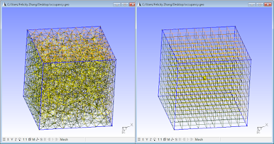
We will fill a simple cube of dimension 1 with cells of characteristic length 0.1, in gmsh (open source, free). I have included below the gmsh (.geo) script used to generate these meshes so that you may play around with the numbers. Here are is a visual comparison:

The results:
Unstructured: 1225 vertices, 6978 elements.
Structured: 1000 vertices, 1331 elements.
Meshing only the faces for a 2D comparison:
Unstructured: 593 vertices, 1297 elements.
Structured: 489 vertices, 603 elements.
So now I am a bit confused about vertices vs. elements. I would have thought 2D elements means 9*9*6 (9 for each dimension, 6 faces) = 486, which is darn close to the vertices count. Hmm if anyone knows please post, and if not in the meantime maybe I will get to updating this.
Interesting fact, I guess there may be some pseudorandomness in the mesh generation; reloading the file and remeshing gave slightly different results. Another element count I got for unstructured 3D meshing was 6624.
The script:
transfinite = 1;//toggle 0 or 1, for unstructured or structured, respectively.
cellLength = 0.1;
cubeLength = 1;
Point(1) = {0,0,0,cellLength};Point(2) = {0,0,cubeLength,cellLength};
Point(3) = {0,cubeLength,0,cellLength};Point(4) = {0,cubeLength,cubeLength,cellLength};
Point(5) = {cubeLength,0,0,cellLength};Point(6) = {cubeLength,0,cubeLength,cellLength};
Point(7) = {cubeLength,cubeLength,0,cellLength};Point(8) = {cubeLength,cubeLength,cubeLength,cellLength};
Point(9) = {0,0,0,cellLength};
Line(1) = {8, 7};
Line(2) = {7, 5};
Line(3) = {5, 6};
Line(4) = {6, 8};
Line(5) = {8, 4};
Line(6) = {4, 2};
Line(7) = {2, 6};
Line(8) = {3, 7};
Line(9) = {3, 4};
Line(10) = {3, 1};
Line(11) = {1, 2};
Line(12) = {1, 5};
Line Loop(13) = {5, -9, 8, -1};
Plane Surface(14) = {13};
Line Loop(15) = {10, 11, -6, -9};
Plane Surface(16) = {15};
Line Loop(17) = {7, 4, 5, 6};
Plane Surface(18) = {17};
Line Loop(19) = {3, 4, 1, 2};
Plane Surface(20) = {19};
Line Loop(21) = {8, 2, -12, -10};
Plane Surface(22) = {21};
Line Loop(23) = {3, -7, -11, 12};
Plane Surface(24) = {23};
Surface Loop(25) = {22, 14, 18, 24, 20, 16};
Volume(26) = {25};
If(transfinite==1)
Transfinite Line {1:12} = cubeLength/cellLength;
Transfinite Surface {14,16,18,20,22,24};
Recombine Surface{14,16,18,20,22,24};
Transfinite Volume {26};
EndIf
Tuesday, March 6, 2012
Hybrid structured/unstructured meshing with Gmsh
I recently became aware of Gmsh's awesome capability to create a hybrid structured-unstructured mesh.

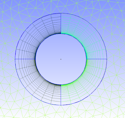
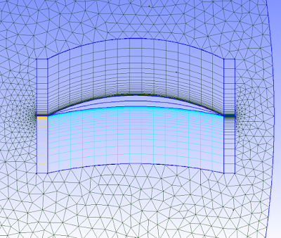
If you are not familiar with these mesh types, unstructured is the one that can be quickly generated around a complex body with the click of a button. The cells turn out triangular in 2D (usually, and can be 4-sided or more) and usually pyramidal in 3D. Structured meshes are made by specifying point locations on an outer rectangular block. Structured mesh cells turn out to be square / rectangular in 2D and rectangular prismatic in 3D. Structured meshes usually take more time than unstructured.
So why use structured? One important flow phenomenon that cannot be efficiently captured by unstructured meshes is boundary layer separation. For drag simulations, predicting boundary layer separation is key. With structured meshes the cells can have a high aspect ratio to have small spacing normal to the wall to resolve the large velocity gradient, and larger spacing parallel to the wall, in which pressure/velocity gradient is not as huge. Unstructured meshes maintain roughly an equilateral shape, and stretching out unstructured mesh cells results in bad mesh quality in terms of skew. So to get boundary-layer resolution with unstructured would take many more cells than with structured cells; structured cells basically allow you to be more efficient with the cells you use.
So many CFD'ers use both unstructured and structured meshes; unstructured as the default, and structured in special areas of interest. Below are a few pictures of part of a hybrid mesh I created in Gmsh (free) for a 2D simulation in OpenFOAM (also free), and it worked perfectly in parallel simulation.


There are tutorial files on the Gmsh website that show you how to do this easily. Look at tutorial file t6.geo. Good luck!
Monday, February 27, 2012
A note about xbee serial communication accuracy
I found a neat fact about the xbee communication modules. Having too high a send rate can botch the accuracy of your transmission (although you should test it yourself, may be just the way my software works). I had two xbees transmitting strings at 57600 baud and quite a bit of noise was present. Turning it down to 4800 resulted in perfect transmission. This is a bit slow, but I will be determining the max transmission rate that doesn't give me noise.
Monday, January 9, 2012
Simple Arduino double-to-string function
Because Arduino language is rather low-level (C-based), such a function is not so straightforward or available as one might think.
Just input the double and the number of decimal places desired. The function:
//Rounds down (via intermediary integer conversion truncation)String doubleToString(double input,int decimalPlaces){if(decimalPlaces!=0){String string = String((int)(input*pow(10,decimalPlaces)));if(abs(input)<1){if(input>0)string = "0"+string;else if(input<0)string = string.substring(0,1)+"0"+string.substring(1);}return string.substring(0,string.length()-decimalPlaces)+"."+string.substring(string.length()-decimalPlaces);}else {return String((int)input);}}
More omniwheel-drive control considerations
Here are some plots and MATLAB code that shows the relationship between the net contribution of the motors versus direction, for different numbers of motors/wheels on the vehicle. The 'net contribution' of the motors was calculated by adding the absolute value of the motor wheel direction (contribution direction) dotted with the direction of the vehicle's movement. The motor usage 'efficiency' is the same figure as described, but divided by the number of motors. An efficiency of 1 would be where all the motors are lined up and going the same direction, which will not happen with an omniwheel vehicle. The efficiency consistently floats around the .6-.7 range, which is pretty good. Meaning if I use 5 of these 135-watt DC motors, I would get about 440 W of rated DC power driving around. Not bad.

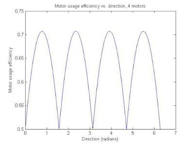
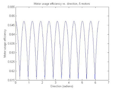
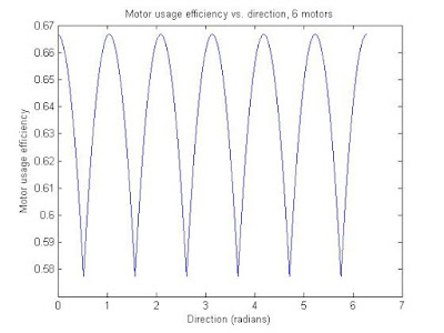
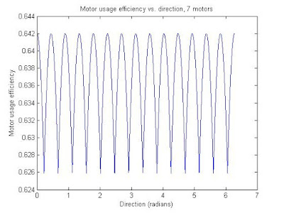
The code also includes last post's stuff (the speed consistency vs. direction plots). Again, even/odd wheel numbers are in their own trend groups, and as the number of motors go up the standard deviation of the efficiency with respect to direction goes down.
The efficiency plots:
The code:
%FPS bot testingclose all;offsetAngles = [0 0 0 0 0];%Just the difference in angle between frontmost motor and forward direction.motorCounts = [3 4 5 6 7];motorAngles = 2*pi./motorCounts;for j = 1:numel(motorCounts)mvec = zeros(motorCounts(j),2);for k = 1:motorCounts(j)mvec(k,:) = [cos(offsetAngles(j)+(k-1)*motorAngles(j)) -sin(offsetAngles(j)+(k-1)*motorAngles(j))];endresolution = 10000;theta = linspace(0,2*pi,resolution)';directionVector = zeros(resolution,2);directionVector(:,1) = cos(theta);directionVector(:,2) = sin(theta);%Speedmag = zeros(resolution,1);currentMag = zeros(motorCounts(j),1);for k=1:resolutionfor i=1:motorCounts(j)currentMag(i) = abs(mvec(i,:)*directionVector(k,:)');endmag(k) = max(currentMag);endfigure;plot(theta,mag);ylabel('Normalized speed magnitude');xlabel('Direction (radians)');title(['Normalized speed magnitude vs. direction, ' num2str(motorCounts(j)) ' motors']);%TorquemotorUse = zeros(resolution,1);for k=1:resolutionfor m=1:motorCounts(j)motorUse(k) = motorUse(k)+abs(mvec(m,:)*directionVector(k,:)');endendfigure;plot(theta,motorUse);ylabel('Equivalent motor usage (# of motors)');xlabel('Direction (radians)');title(['Motor usage vs. direction, ' num2str(motorCounts(j)) ' motors']);figure;plot(theta,motorUse/motorCounts(j));ylabel('Motor usage efficiency');xlabel('Direction (radians)');title(['Motor usage efficiency vs. direction, ' num2str(motorCounts(j)) ' motors']);end
Thursday, January 5, 2012
Timing Pulley Transmission Calculator
Here is a nice calculator for setting up a new timing pulley transmission: http://www.sdp-si.com/cd/default.htm. It takes into account pulley center distance, belt sizes, pitch, speed ratio, and pulley tooth requirements. The nice thing is that the choices of materials is based on what is in stock at SDP/SI. I have ordered from them a few times.
Sunday, January 1, 2012
Changing Arduino Output PWM frequency
Here is a very useful post about changing the output PWM frequency on the Arduino (post #5). It was useful for me because I wanted a frequency over 20 kHz for DC motor control (>20 kHz is above the hearing range).
Getting PWM frequency and duty cycle with Arduino
Here is a simple code that reads a PWM signal and calculates its frequency and duty cycle in real time. The lack of an oscilloscope motivated this code.
The star of the show is the built-in 'pulseIn()' function, which gives the length of a low or high pulse. With these two measurements the calculation of duty cycle and frequency of the PWM signal is straightforward.
I have two different versions, simple and slightly longer.
The slightly longer code takes a user-specified time delay over which the maximum length is taken to help prevent truncation of a signal. For example, if an input pulse of 10 ms has already been running for 2 ms and the pulseIn function is called, it may return 8 ms. I am actually not sure if this is the way pulseIn works, but I tried both. With the default Arduino PWM frequency of approximately 490 Hz (http://arduino.cc/en/Reference/analogWrite), the slightly longer code returns 490 +/- 3 Hz, while the simple code returns 500 +/- 3 Hz. I tested this over low and high duty cycles. So it appears the slightly longer code has slightly better accuracy.
Simple code:
//Reads a PWM signal's duty cycle and frequency.#define READ_PIN 13#define PWM_OUTPUT 10static double duty;static double freq;static long highTime = 0;static long lowTime = 0;static long tempPulse;void setup(){pinMode(READ_PIN,INPUT);Serial.begin(9600);analogWrite(PWM_OUTPUT,230);}void loop(){readPWM(READ_PIN);Serial.println(freq);Serial.println(duty);}//Takes in reading pins and outputs pwm frequency and duty cycle.void readPWM(int readPin){highTime = 0;lowTime = 0;tempPulse = pulseIn(readPin,HIGH);if(tempPulse>highTime){highTime = tempPulse;}tempPulse = pulseIn(readPin,LOW);if(tempPulse>lowTime){lowTime = tempPulse;}freq = ((double) 1000000)/(double (lowTime+highTime));duty = (100*(highTime/(double (lowTime+highTime))));}
Slightly longer code:
//Reads a PWM signal's duty cycle and frequency.#define READ_PIN 13#define READ_DELAY 100#define PWM_OUTPUT 10static double duty;static double freq;static long highTime = 0;static long lowTime = 0;static long tempPulse;static long lastSeen;void setup(){pinMode(READ_PIN,INPUT);Serial.begin(9600);analogWrite(PWM_OUTPUT,230);}void loop(){readPWM(READ_PIN);Serial.println(freq);Serial.println(duty);}//Takes in reading pins and outputs pwm frequency and duty cycle.void readPWM(int readPin){highTime = 0;lowTime = 0;lastSeen = millis();while((millis()-lastSeen)<read_delay){< div="">tempPulse = pulseIn(readPin,HIGH);if(tempPulse>highTime){highTime = tempPulse;}}lastSeen = millis();while((millis()-lastSeen)<read_delay){< div="">tempPulse = pulseIn(readPin,LOW);if(tempPulse>lowTime){lowTime = tempPulse;}}freq = ((double) 1000000)/(double (lowTime+highTime));duty = (100*(highTime/(double (lowTime+highTime))));}
Subscribe to:
Posts (Atom)